Summary Analysis

Coin catalogue sections:	Holmoi, Kelenderis, Pseudo-Kelenderis Mints
Coin corpus datasets:	Holmoi, Group 1, Holmoi, Group 2, Kelenderis, staters, Group 1, Kelenderis, staters, Group 2, Kelenderis, staters, Group 3, Pseudo-Kelenderis Mints

Summary

Silver staters minted at Holmoi, Kelenderis and Pseudo-Kelenderis mints can be divided into three large groups based on their weights, which probably correspond to the three phases of the weight standard development in Cilicia Trachea. This relative chronology of stater coinage is based on the assumption that the weight standards used at these mints were synchronous in time.

Analysis

Based on the Coin Catalogue and weight analyses of Holmoi, Kelenderis and Pseudo-Kelenderis mints, silver staters can be divided into the following groups, which group together coin types with the same weight standard:

Holmoi:	Group 1:	Type 1;
	Group 2:	Type 2.
Kelenderis:	Group 1:	Types 1.1–3;
	Group 2:	Types 2.1–12;
	Group 3A:	Types 3.1–3 and 3.7–12;
	Group 3B:	Types 3.13–14;
	Group 3C:	Types 3.4–6 and 3.15–17.
Pseudo-Kelenderis:	Group 1:	Type 1;
	Group 2:	Type 2.

Box plots1, cumulative distributions and basic descriptive statistics of these groups are presented in Figures 1–2 and Table 1 (Std. Dev. denotes the standard deviation and IQR the interquartile range), respectively.

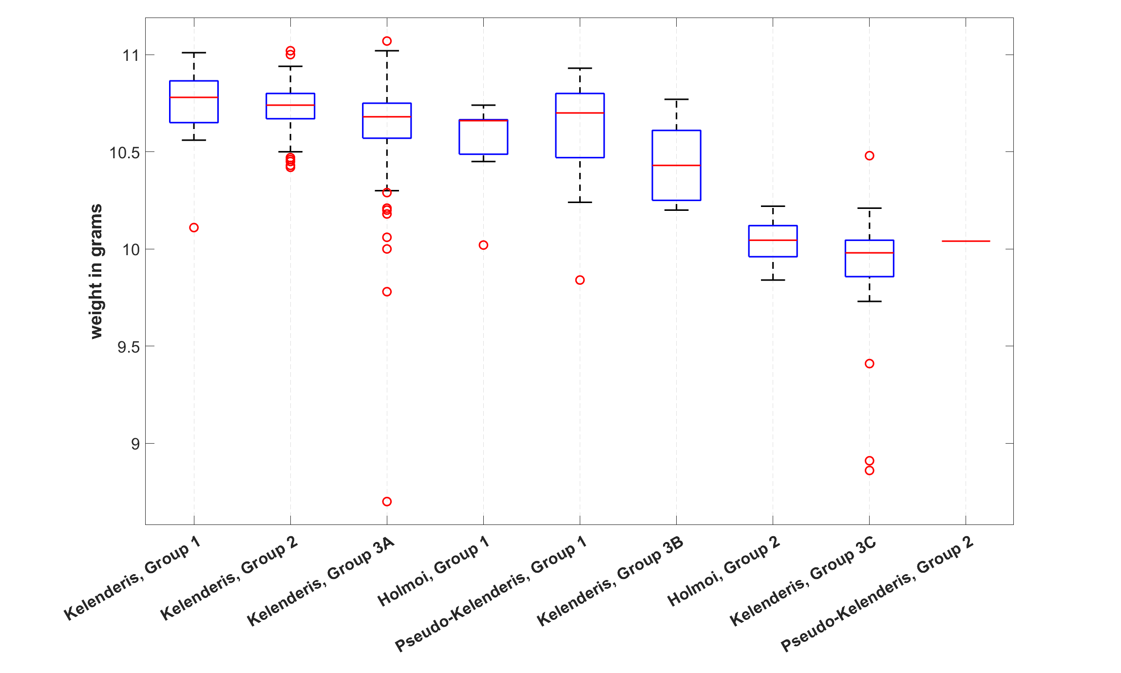
Figure 1: Box plots of individual groups of staters

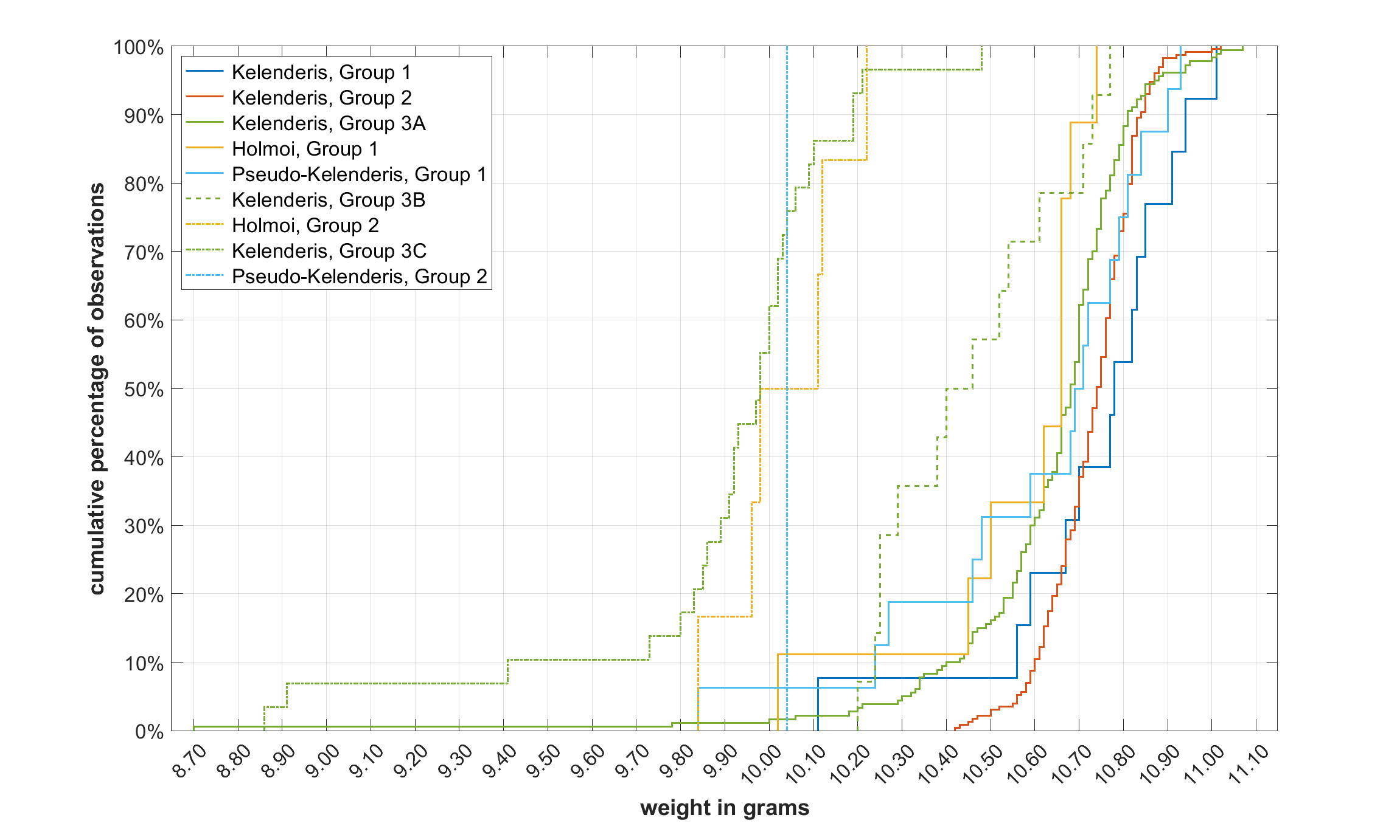
Figure 2: Cumulative distributions of individual groups of staters

Group	Count	Mean	Median	Std. Dev.	IQR
Kelenderis, Group 1	13	10.73	10.78	0.23	0.21
Kelenderis, Group 2	229	10.73	10.74	0.10	0.13
Kelenderis, Group 3A	180	10.64	10.68	0.23	0.18
Holmoi, Group 1	9	10.55	10.66	0.22	0.18
Pseudo-Kelenderis, Group 1	16	10.61	10.70	0.29	0.33
Kelenderis, Group 3B	14	10.45	10.43	0.20	0.36
Holmoi, Group 2	6	10.04	10.04	0.14	0.16
Kelenderis, Group 3C	29	9.90	9.98	0.34	0.19
Pseudo-Kelenderis, Group 2	1	10.04	10.04	0.00	0.00

Table 1: Basic descriptive statistics of individual groups of staters

As Figures 1–2 and Table 1 show, the staters of these mints can be divided in terms of the similarity of their weights into three large groups, which probably correspond to the three phases of the weight standard development in Cilicia Trachea:

Phase 1:	Holmoi, Group 1; Kelenderis, Groups 1, 2 and 3A; Pseudo-Kelenderis, Group 1.
Phase 2:	Kelenderis, Group 3B.
Phase 3:	Holmoi, Group 2; Kelenderis, Group 3C; Pseudo-Kelenderis, Group 2.

Box plots and descriptive statistics of these three assumed phases are presented in Figure 3 and Table 2, respectively. In Table 2, note the large negative skewness of Phases 1 and 3, which is manifested in Figure 3 by high numbers of outliers below the bottom whiskers. The weight distributions of these two phases are considerably left-skewed.

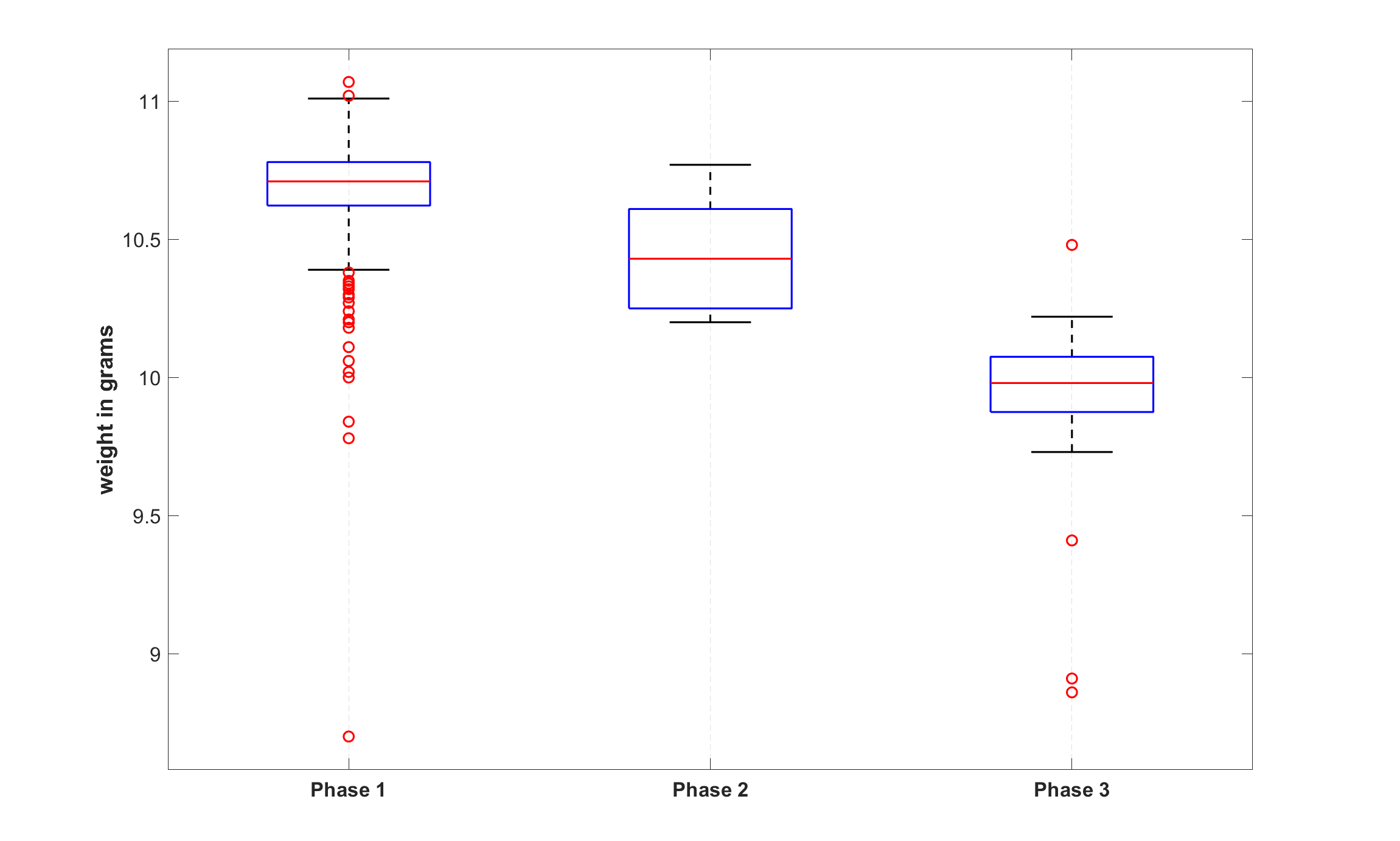
Figure 3: Box plots of phases of weight standard development

Statistics	Phase 1	Phase 2	Phase 3
Number of coins:	447	14	36
Mean:	10.68	10.45	9.93
Standard deviation:	0.18	0.20	0.31
Interquartile range:	0.16	0.36	0.20
Skewness:	-3.85	0.28	-2.10
Kurtosis:	34.90	1.71	8.25
Minimum:	8.70	10.20	8.86
25th percentile:	10.62	10.25	9.88
Median:	10.71	10.43	9.98
75th percentile:	10.78	10.61	10.07
Maximum:	11.07	10.77	10.48

Table 2: Descriptive statistics of phases of weight standard development

Figure 4 presents relative frequency histograms. The bars represent the relative frequencies of observations ranging from 8.70 to 11.10 g in increments of 0.10 g and the continuous curves represent approximations of the data by the Weibull distribution2 based on maximum likelihood estimates. Cumulative distributions are shown in Figure 5.

Figure 4: Relative frequency histograms of phases of weight standard development

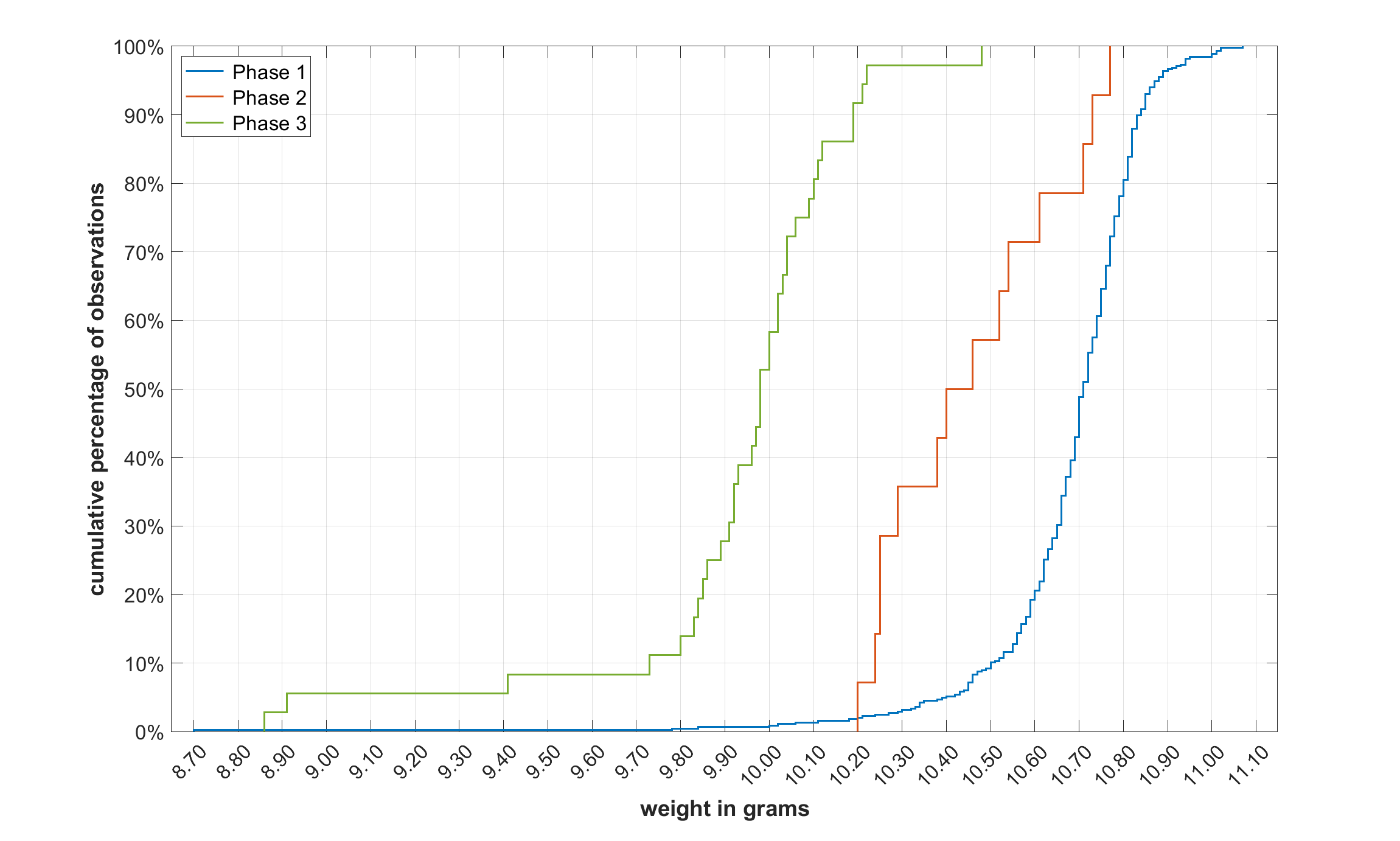
Figure 5: Cumulative distributions of phases of weight standard development

The distributions of coin weights in individual groups have different shapes and are asymmetric. Instead of comparing means, it is therefore statistically more appropriate to compare medians. Since the analyzed data have many tied values, the percentile bootstrap method was chosen. Table 3 shows the observed sample medians and bootstrap 95% confidence intervals.3 Table 4 shows the differences in sample medians, their bootstrap 95% confidence intervals and p-values.4 These results confirm that the weight distributions of Phases 1, 2 and 3 are significantly different at the 5% significance level.

	median	95% confidence interval
Phase 1	10.71	10.70	10.72
Phase 2	10.43	10.27	10.61
Phase 3	9.98	9.92	10.03

Table 3: Medians and their confidence intervals

	medians difference	95% confidence interval		p-value
Phase 1 vs Phase 2	0.28	0.11	0.45	0.004
Phase 1 vs Phase 3	0.73	0.68	0.79	<0.001
Phase 2 vs Phase 3	0.45	0.27	0.62	<0.001

Table 4: Differences in medians